Fast GeoSpatial Analysis in Python
This work is supported by Anaconda Inc., the Data Driven Discovery Initiative from the Moore Foundation, and NASA SBIR NNX16CG43P
This work is a collaboration with Joris Van den Bossche. This blogpost builds on Joris’s EuroSciPy talk (slides) on the same topic. You can also see Joris’ blogpost on this same topic.
TL;DR:
Python’s Geospatial stack is slow. We accelerate the GeoPandas library with Cython and Dask. Cython provides 10-100x speedups. Dask gives an additional 3-4x on a multi-core laptop. Everything is still rough, please come help.
We start by reproducing a blogpost published last June, but with 30x speedups. Then we talk about how we achieved the speedup with Cython and Dask.
All code in this post is experimental. It should not be relied upon.
Experiment
In June Ravi Shekhar published a blogpost Geospatial Operations at Scale with Dask and GeoPandas in which he counted the number of rides originating from each of the official taxi zones of New York City. He read, processed, and plotted 120 million rides, performing an expensive point-in-polygon test for each ride, and produced a figure much like the following:
This took about three hours on his laptop. He used Dask and a bit of custom code to parallelize Geopandas across all of his cores. Using this combination he got close to the speed of PostGIS, but from Python.
Today, using an accelerated GeoPandas and a new dask-geopandas library, we can do the above computation in around eight minutes (half of which is reading CSV files) and so can produce a number of other interesting images with faster interaction times.
A full notebook producing these plots is available below:
The rest of this article talks about GeoPandas, Cython, and speeding up geospatial data analysis.
Background in Geospatial Data
The Shapely User Manual begins with the following passage on the utility of geospatial analysis to our society.
Deterministic spatial analysis is an important component of computational approaches to problems in agriculture, ecology, epidemiology, sociology, and many other fields. What is the surveyed perimeter/area ratio of these patches of animal habitat? Which properties in this town intersect with the 50-year flood contour from this new flooding model? What are the extents of findspots for ancient ceramic wares with maker’s marks “A” and “B”, and where do the extents overlap? What’s the path from home to office that best skirts identified zones of location based spam? These are just a few of the possible questions addressable using non-statistical spatial analysis, and more specifically, computational geometry.
Shapely is part of Python’s GeoSpatial stack which is currently composed of the following libraries:
- Shapely: Manages shapes like points, linestrings, and polygons. Wraps the GEOS C++ library
- Fiona: Handles data ingestion. Wraps the GDAL library
- Rasterio: Handles raster data like satelite imagery
- GeoPandas: Extends Pandas with a column of shapely geometries to intuitively query tables of geospatially annotated data.
These libraries provide intuitive Python wrappers around the OSGeo C/C++ libraries (GEOS, GDAL, …) which power virtually every open source geospatial library, like PostGIS, QGIS, etc.. They provide the same functionality, but are typically much slower due to how they use Python. This is acceptable for small datasets, but becomes an issue as we transition to larger and larger datasets.
In this post we focus on GeoPandas, a geospatial extension of Pandas which manages tabular data that is annotated with geometry information like points, paths, and polygons.
GeoPandas Example
GeoPandas makes it easy to load, manipulate, and plot geospatial data. For example, we can download the NYC taxi zones, load and plot them in a single line of code.
geopandas.read_file('taxi_zones.shp')
         .to_crs({'init' :'epsg:4326'})
         .plot(column='borough', categorical=True)

Cities are now doing a wonderful job publishing data into the open. This provides transparency and an opportunity for civic involvement to help analyze, understand, and improve our communities. Here are a few fun geospatially-aware datasets to make you interested:
- Chicago Crimes from 2001 to present (one week ago)
- Paris Velib (bikeshare) in real time
- Bike lanes in New Orleans
- New Orleans Police Department incidents involving the use of force
Performance
Unfortunately GeoPandas is slow. This limits interactive exploration on larger datasets. For example the Chicago crimes data (the first dataset above) has seven million entries and is several gigabytes in memory. Analyzing a dataset of this size interactively with GeoPandas is not feasible today.

This slowdown is because GeoPandas wraps each geometry (like a point, line, or
polygon) with a Shapely object and stores all of those objects in an
object-dtype column. When we compute a GeoPandas operation on all of our
shapes we just iterate over these shapes in Python. As an example, here is how
one might implement a distance method in GeoPandas today.
def distance(self, other):
    result = [geom.distance(other)
              for geom in self.geometry]
    return pd.Series(result)
Unfortunately this just iterates over elements in the series, each of which is an individual Shapely object. This is inefficient for two reasons:
- Iterating through Python objects is slow relative to iterating through those same objects in C.
- Shapely Python objects consume more memory than the GEOS Geometry objects that they wrap.
This results in slow performance.
Cythonizing GeoPandas
Fortunately, we’ve rewritten GeoPandas with Cython to directly loop over the
underlying GEOS pointers. This provides a 10-100x speedup depending on the
operation.
So instead of using a Pandas object-dtype column that holds shapely objects
we instead store a NumPy array of direct pointers to the GEOS objects.
Before
After

As an example, our function for distance now looks like the following Cython implementation (some liberties taken for brevity):
cpdef distance(self, other):
    cdef int n = self.size
    cdef GEOSGeometry *left_geom
    cdef GEOSGeometry *right_geom = other.__geom__  # a geometry pointer
    geometries = self._geometry_array

    with nogil:
        for idx in xrange(n):
            left_geom = <GEOSGeometry *> geometries[idx]
            if left_geom != NULL:
                distance = GEOSDistance_r(left_geom, some_point.__geom)
            else:
                distance = NaN
For fast operations we see speedups of 100x. For slower operations we’re closer to 10x. Now these operations run at full C speed.
In his EuroSciPy talk Joris compares the performance of GeoPandas (both before and after Cython) with PostGIS, the standard geospatial plugin for the popular PostgreSQL database (original notebook with the comparison). I’m stealing some plots from his talk below:
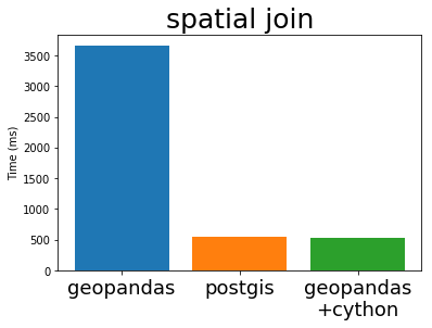
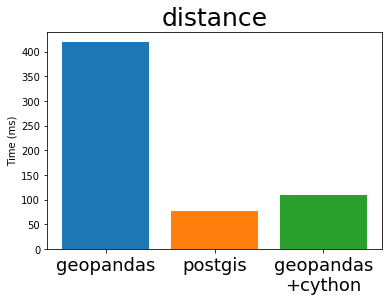
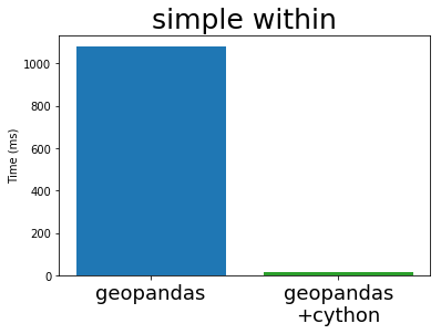
Cythonized GeoPandas and PostGIS run at almost exactly the same speed. This is because they use the same underlying C library, GEOS. These algorithms are not particularly complex, so it is not surprising that everyone implements them in exactly the same way.
This is great. The Python GIS stack now has a full-speed library that operates as fast as any other open GIS system is likely to manage.
Problems
However, this is still a work in progress, and there is still plenty of work to do.
First, we need for Pandas to track our arrays of GEOS pointers differently from how it tracks a normal integer array. This is both for usability reasons, like we want to render them differently and don’t want users to be able to perform numeric operations like sum and mean on these arrays, and also for stability reasons, because we need to track these pointers and release their allocated GEOSGeometry objects from memory at the appropriate times. Currently, this goal is pursued by creating a new block type, the GeometryBlock (‘blocks’ are the internal building blocks of pandas that hold the data of the different columns). This will require some changes to Pandas itself to enable custom block types (see this issue on the pandas issue tracker).
Second, data ingestion is still quite slow. This relies not on GEOS, but on GDAL/OGR, which is handled in Python today by Fiona. Fiona is more optimized for consistency and usability rather than raw speed. Previously when GeoPandas was slow this made sense because no one was operating on particularly large datasets. However now we observe that data loading is often several times more expensive than all of our manipulations so this will probably need some effort in the future.
Third, there are some algorithms within GeoPandas that we haven’t yet Cythonized. This includes both particular features like overlay and dissolve operations as well as small components like GeoJSON output.
Finally as with any rewrite on a codebase that is not exhaustively tested (we’re trying to improve testing as we do this) there are probably several bugs that we won’t detect until some patient and forgiving user runs into them first.
Still though, all linear geospatial operations work well and are thoroughly tested. Also spatial joins (a backbone of many geospatial operations) are up and running at full speed. If you work in a non-production environment then Cythonized GeoPandas may be worth your time to investigate.
You can track future progress on this effort at geopandas/geopandas #473 which includes installation instructions.
Parallelize with Dask
Cythonizing gives us speedups in the 10x-100x range. We use a single core as effectively as is possible with the GEOS library. Now we move on to using multiple cores in parallel. This gives us an extra 3-4x on a standard 4 core laptop. We can also scale to clusters, though I’ll leave that for a future blogpost.
To parallelize we need to split apart our dataset into multiple chunks. We can do this naively by placing the first million rows in one chunk, the second million rows in another chunk, etc. or we can partition our data spatially, for example by placing all of the data for one region of our dataset in one chunk and all of the data for another region in another chunk, and so on. Both approaches are implemented in a rudimentary dask-geopandas library available on GitHub.
So just as dask-array organizes many NumPy arrays along a grid and dask-dataframe organizes many Pandas dataframes along a linear index


the dask-geopandas library organizes many GeoPandas dataframes into spatial regions. In the example below we might partition data in the city of New York into its different boroughs. Data for each borough would be handled separately by a different thread or, in a distributed situation, might live on a different machine.

This gives us two advantages:
- Even without geospatial partitioning, we can use many cores (or many machines) to accelerate simple operations.
- For spatially aware operations, like spatial joins or subselections we can engage only those parts of the parallel dataframe that we know are relevant for various parts of the computation.
However this is also expensive and not always necessary. In our initial exercise with the NYC Taxi data we didn’t do this, and will still got significant speedups just from normal multicore operation.
Exercise
And so to produce the images we did at the top of this post we used a combination of dask.dataframe to load in CSV files, dask-geopandas to perform the spatial join, and then dask.dataframe and normal pandas to perform the actual computations. Our code looked something like the following:
import dask.dataframe as dd
import dask_geopandas as dg

df = dd.read_csv('yellow_tripdata_2015-*.csv')
gf = dg.set_geometry(df, geometry=df[['pickup_longitude', 'pickup_latitude']],
                     crs={'init' :'epsg:4326'})
gf = dg.sjoin(gf, zones[['zone', 'borough', 'geometry']])
full = gf[['zone', 'payment_type', 'tip_amount', 'fare_amount']]

full.to_parquet('nyc-zones.parquet')  # compute and cache result on disk
full = dd.read_parquet('nyc-zones.parquet')
And then we can do typical groupbys and joins on the more typical pandas-like data now properly annotated with zones.
result = full.passenger_count.groupby(full.zone).count().compute()
result.name = 'count'
joined = pd.merge(result.to_frame(), zones,
                  left_index=True, right_on='zone')
joined = geopandas.GeoDataFrame(joined)  # convert back for plotting
We’ve replaced most of Ravi’s custom analysis with a few lines of new standard code. This maxes our or CPU when doing spatial joins. Everything here releases the GIL well and the entire computation operates in under a couple gigabytes of RAM.
Problems
The dask-geopandas project is currently a prototype. It will easily break for non-trivial applications (and indeed many trivial ones). It was designed to see how hard it would be to implement some of the trickier operations like spatial joins, repartitioning, and overlays. This is why, for example, it supports a fully distributed spatial join, but lacks simple operations like indexing. There are other longer-term issues as well.
Serialization costs are manageable, but decently high. We currently use the standard “well known binary” WKB format common in other geospatial applications but have found it to be fairly slow, which bogs down inter-process parallelism.
Similarly distributed and spatially partitioned data stores don’t seem to be common (or at least I haven’t run across them yet).
It’s not clear how dask-geopandas dataframes and normal dask dataframes should interact. It would be very convenient to reuse all of the algorithms in dask.dataframe, but the index structures of the two libraries is very different. This may require some clever software engineering on the part of the Dask developers.
Still though, these seem surmountable and generally this process has been easy so far. I suspect that we can build an intuitive and performant parallel GIS analytics system with modest effort.
The notebook for the example at the start of the blogpost shows using dask-geopandas with good results.
Conclusion
With established technologies in the PyData space like Cython and Dask we’ve been able to accelerate and scale GeoPandas operations above and beyond industry standards. However this work is still experimental and not ready for production use. This work is a bit of a side project for both Joris and Matthew and they would welcome effort from other experienced open source developers. We believe that this project can have a large social impact and are enthusiastic about pursuing it in the future. We hope that you share our enthusiasm.
- NYC Taxi GeoSpatial Analysis Notebook
- Joris’s EuroSciPy talk
- Joris’s blogpost
- Ravi’s original post Geospatial Operations at Scale with Dask and GeoPandas
blog comments powered by Disqus