Pandas on HDFS with Dask Dataframes
This work is supported by Continuum Analytics and the XDATA Program as part of the Blaze Project
In this post we use Pandas in parallel across an HDFS cluster to read CSV data. We coordinate these computations with dask.dataframe. A screencast version of this blogpost is available here and the previous post in this series is available here.
To start, we connect to our scheduler, import the hdfs module from the
distributed library, and read our CSV data from HDFS.
>>> from distributed import Executor, hdfs, progress
>>> e = Executor('127.0.0.1:8786')
>>> e
<Executor: scheduler=127.0.0.1:8786 workers=64 threads=64>

>>> nyc2014 = hdfs.read_csv('/nyctaxi/2014/*.csv',
...               parse_dates=['pickup_datetime', 'dropoff_datetime'],
...               skipinitialspace=True)

>>> nyc2015 = hdfs.read_csv('/nyctaxi/2015/*.csv',
...               parse_dates=['tpep_pickup_datetime', 'tpep_dropoff_datetime'])

>>> nyc2014, nyc2015 = e.persist([nyc2014, nyc2015])
>>> progress(nyc2014, nyc2015)
Our data comes from the New York City Taxi and Limousine Commission which publishes all yellow cab taxi rides in NYC for various years. This is a nice model dataset for computational tabular data because it’s large enough to be annoying while also deep enough to be broadly appealing. Each year is about 25GB on disk and about 60GB in memory as a Pandas DataFrame.
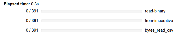
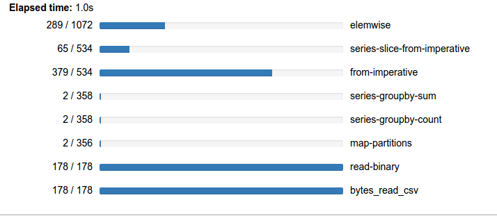
HDFS breaks up our CSV files into 128MB chunks on various hard drives spread
throughout the cluster. The dask.distributed workers each read the chunks of
bytes local to them and call the pandas.read_csv function on these bytes,
producing 391 separate Pandas DataFrame objects spread throughout the memory of
our eight worker nodes. The returned objects, nyc2014 and nyc2015, are
dask.dataframe objects which
present a subset of the Pandas API to the user, but farm out all of the work to
the many Pandas dataframes they control across the network.
Play with Distributed Data
If we wait for the data to load fully into memory then we can perform pandas-style analysis at interactive speeds.
>>> nyc2015.head()
| VendorID | tpep_pickup_datetime | tpep_dropoff_datetime | passenger_count | trip_distance | pickup_longitude | pickup_latitude | RateCodeID | store_and_fwd_flag | dropoff_longitude | dropoff_latitude | payment_type | fare_amount | extra | mta_tax | tip_amount | tolls_amount | improvement_surcharge | total_amount | |
|---|---|---|---|---|---|---|---|---|---|---|---|---|---|---|---|---|---|---|---|
| 0 | 2 | 2015-01-15 19:05:39 | 2015-01-15 19:23:42 | 1 | 1.59 | -73.993896 | 40.750111 | 1 | N | -73.974785 | 40.750618 | 1 | 12.0 | 1.0 | 0.5 | 3.25 | 0 | 0.3 | 17.05 |
| 1 | 1 | 2015-01-10 20:33:38 | 2015-01-10 20:53:28 | 1 | 3.30 | -74.001648 | 40.724243 | 1 | N | -73.994415 | 40.759109 | 1 | 14.5 | 0.5 | 0.5 | 2.00 | 0 | 0.3 | 17.80 |
| 2 | 1 | 2015-01-10 20:33:38 | 2015-01-10 20:43:41 | 1 | 1.80 | -73.963341 | 40.802788 | 1 | N | -73.951820 | 40.824413 | 2 | 9.5 | 0.5 | 0.5 | 0.00 | 0 | 0.3 | 10.80 |
| 3 | 1 | 2015-01-10 20:33:39 | 2015-01-10 20:35:31 | 1 | 0.50 | -74.009087 | 40.713818 | 1 | N | -74.004326 | 40.719986 | 2 | 3.5 | 0.5 | 0.5 | 0.00 | 0 | 0.3 | 4.80 |
| 4 | 1 | 2015-01-10 20:33:39 | 2015-01-10 20:52:58 | 1 | 3.00 | -73.971176 | 40.762428 | 1 | N | -74.004181 | 40.742653 | 2 | 15.0 | 0.5 | 0.5 | 0.00 | 0 | 0.3 | 16.30 |
>>> len(nyc2014)
165114373

>>> len(nyc2015)
146112989
Interestingly it appears that the NYC cab industry has contracted a bit in the last year. There are fewer cab rides in 2015 than in 2014.
When we ask for something like the length of the full dask.dataframe we actually ask for the length of all of the hundreds of Pandas dataframes and then sum them up. This process of reaching out to all of the workers completes in around 200-300 ms, which is generally fast enough to feel snappy in an interactive session.
The dask.dataframe API looks just like the Pandas API, except that we call
.compute() when we want an actual result.
>>> nyc2014.passenger_count.sum().compute()
279997507.0

>>> nyc2015.passenger_count.sum().compute()
245566747
Dask.dataframes build a plan to get your result and the distributed scheduler coordinates that plan on all of the little Pandas dataframes on the workers that make up our dataset.
Pandas for Metadata
Let’s appreciate for a moment all the work we didn’t have to do around CSV handling because Pandas magically handled it for us.
>>> nyc2015.dtypes
VendorID                          int64
tpep_pickup_datetime     datetime64[ns]
tpep_dropoff_datetime    datetime64[ns]
passenger_count                   int64
trip_distance                   float64
pickup_longitude                float64
pickup_latitude                 float64
RateCodeID                        int64
store_and_fwd_flag               object
dropoff_longitude               float64
dropoff_latitude                float64
payment_type                      int64
fare_amount                     float64
extra                           float64
mta_tax                         float64
tip_amount                      float64
tolls_amount                    float64
improvement_surcharge           float64
total_amount\r                  float64
dtype: object
We didn’t have to find columns or specify data-types. We didn’t have to parse
each value with an int or float function as appropriate. We didn’t have to
parse the datetimes, but instead just specified a parse_datetimes= keyword.
The CSV parsing happened about as quickly as can be expected for this format,
clocking in at a network total of a bit under 1 GB/s.
Pandas is well loved because it removes all of these little hurdles from the life of the analyst. If we tried to reinvent a new “Big-Data-Frame” we would have to reimplement all of the work already well done inside of Pandas. Instead, dask.dataframe just coordinates and reuses the code within the Pandas library. It is successful largely due to work from core Pandas developers, notably Masaaki Horikoshi (@sinhrks), who have done tremendous work to align the API precisely with the Pandas core library.
Analyze Tips and Payment Types
In an effort to demonstrate the abilities of dask.dataframe we ask a simple question of our data, “how do New Yorkers tip?”. The 2015 NYCTaxi data is quite good about breaking down the total cost of each ride into the fare amount, tip amount, and various taxes and fees. In particular this lets us measure the percentage that each rider decided to pay in tip.
>>> nyc2015[['fare_amount', 'tip_amount', 'payment_type']].head()
| fare_amount | tip_amount | payment_type | |
|---|---|---|---|
| 0 | 12.0 | 3.25 | 1 |
| 1 | 14.5 | 2.00 | 1 |
| 2 | 9.5 | 0.00 | 2 |
| 3 | 3.5 | 0.00 | 2 |
| 4 | 15.0 | 0.00 | 2 |
In the first two lines we see evidence supporting the 15-20% tip standard
common in the US. The following three lines interestingly show zero tip.
Judging only by these first five lines (a very small sample) we see a strong
correlation here with the payment type. We analyze this a bit more by counting
occurrences in the payment_type column both for the full dataset, and
filtered by zero tip:
>>> %time nyc2015.payment_type.value_counts().compute()
CPU times: user 132 ms, sys: 0 ns, total: 132 ms
Wall time: 558 ms

1    91574644
2    53864648
3      503070
4      170599
5          28
Name: payment_type, dtype: int64

>>> %time nyc2015[nyc2015.tip_amount == 0].payment_type.value_counts().compute()
CPU times: user 212 ms, sys: 4 ms, total: 216 ms
Wall time: 1.69 s

2    53862557
1     3365668
3      502025
4      170234
5          26
Name: payment_type, dtype: int64
We find that almost all zero-tip rides correspond to payment type 2, and that almost all payment type 2 rides don’t tip. My un-scientific hypothesis here is payment type 2 corresponds to cash fares and that we’re observing a tendancy of drivers not to record cash tips. However we would need more domain knowledge about our data to actually make this claim with any degree of authority.
Analyze Tips Fractions
Lets make a new column, tip_fraction, and then look at the average of this
column grouped by day of week and grouped by hour of day.
First, we need to filter out bad rows, both rows with this odd payment type,
and rows with zero fare (there are a surprising number of free cab rides in
NYC.) Second we create a new column equal to the ratio of tip_amount /
fare_amount.
>>> df = nyc2015[(nyc2015.fare_amount > 0) & (nyc2015.payment_type != 2)]
>>> df = df.assign(tip_fraction=(df.tip_amount / df.fare_amount))
Next we choose to groupby the pickup datetime column in order to see how the average tip fraction changes by day of week and by hour. The groupby and datetime handling of Pandas makes these operations trivial.
>>> dayofweek = df.groupby(df.tpep_pickup_datetime.dt.dayofweek).tip_fraction.mean()
>>> hour = df.groupby(df.tpep_pickup_datetime.dt.hour).tip_fraction.mean()

>>> dayofweek, hour = e.persist([dayofweek, hour])
>>> progress(dayofweek, hour)
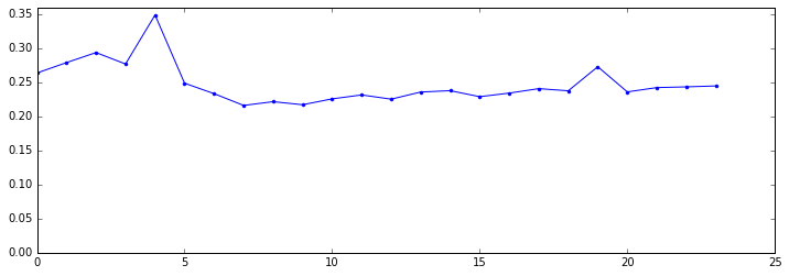
Grouping by day-of-week doesn’t show anything too striking to my eye. However I would like to note at how generous NYC cab riders seem to be. A 23-25% tip can be quite nice:
>>> dayofweek.compute()
tpep_pickup_datetime
0    0.237510
1    0.236494
2    0.236073
3    0.246007
4    0.242081
5    0.232415
6    0.259974
Name: tip_fraction, dtype: float64
But grouping by hour shows that late night and early morning riders are more likely to tip extravagantly:
>>> hour.compute()
tpep_pickup_datetime
0     0.263602
1     0.278828
2     0.293536
3     0.276784
4     0.348649
5     0.248618
6     0.233257
7     0.216003
8     0.221508
9     0.217018
10    0.225618
11    0.231396
12    0.225186
13    0.235662
14    0.237636
15    0.228832
16    0.234086
17    0.240635
18    0.237488
19    0.272792
20    0.235866
21    0.242157
22    0.243244
23    0.244586
Name: tip_fraction, dtype: float64
In [24]:
We plot this with matplotlib and see a nice trough during business hours with a surge in the early morning with an astonishing peak of 34% at 4am:
Performance
Lets dive into a few operations that run at different time scales. This gives a good understanding of the strengths and limits of the scheduler.
>>> %time nyc2015.head()
CPU times: user 4 ms, sys: 0 ns, total: 4 ms
Wall time: 20.9 ms
This head computation is about as fast as a film projector. You could perform this roundtrip computation between every consecutive frame of a movie; to a human eye this appears fluid. In the last post we asked about how low we could bring latency. In that post we were running computations from my laptop in California and so were bound by transcontinental latencies of 200ms. This time, because we’re operating from the cluster, we can get down to 20ms. We’re only able to be this fast because we touch only a single data element, the first partition. Things change when we need to touch the entire dataset.
>>> %time len(nyc2015)
CPU times: user 48 ms, sys: 0 ns, total: 48 ms
Wall time: 271 ms
The length computation takes 200-300 ms. This computation takes longer because we
touch every individual partition of the data, of which there are 178. The
scheduler incurs about 1ms of overhead per task, add a bit of latency
and you get the ~200ms total. This means that the scheduler will likely be the
bottleneck whenever computations are very fast, such as is the case for
computing len. Really, this is good news; it means that by improving the
scheduler we can reduce these durations even further.
If you look at the groupby computations above you can add the numbers in the progress bars to show that we computed around 3000 tasks in around 7s. It looks like this computation is about half scheduler overhead and about half bound by actual computation.
Conclusion
We used dask+distributed on a cluster to read CSV data from HDFS into a dask dataframe. We then used dask.dataframe, which looks identical to the Pandas dataframe, to manipulate our distributed dataset intuitively and efficiently.
We looked a bit at the performance characteristics of simple computations.
What doesn’t work
As always I’ll have a section like this that honestly says what doesn’t work well and what I would have done with more time.
-
Dask dataframe implements a commonly used subset of Pandas functionality, not all of it. It’s surprisingly hard to communicate the exact bounds of this subset to users. Notably, in the distributed setting we don’t have a shuffle algorithm, so
groupby(...).apply(...)and some joins are not yet possible. -
If you want to use threads, you’ll need Pandas 0.18.0 which, at the time of this writing, was still in release candidate stage. This Pandas release fixes some important GIL related issues.
-
The 1ms overhead per task limit is significant. While we can still scale out to clusters far larger than what we have here, we probably won’t be able to strongly accelerate very quick operations until we reduce this number.
-
We use the hdfs3 library to read data from HDFS. This library seems to work great but is new and could use more active users to flush out bug reports.
Links
- dask, the original project
- dask.distributed, the distributed memory scheduler powering the cluster computing
- dask.dataframe, the user API we’ve used in this post.
- NYC Taxi Data Downloads
- hdfs3: Python library we use for HDFS interations.
- The previous post in this blog series.
Setup and Data
You can obtain public data from the New York City Taxi and Limousine Commission here. I downloaded this onto the head node and dumped it into HDFS with commands like the following:
$ wget https://storage.googleapis.com/tlc-trip-data/2015/yellow_tripdata_2015-{01..12}.csv
$ hdfs dfs -mkdir /nyctaxi
$ hdfs dfs -mkdir /nyctaxi/2015
$ hdfs dfs -put yellow*.csv /nyctaxi/2015/
The cluster was hosted on EC2 and was comprised of nine m3.2xlarges with 8
cores and 30GB of RAM each. Eight of these nodes were used as workers; they
used processes for parallelism, not threads.
blog comments powered by Disqus