SymPy and Theano -- Code Generation

No one is good at everything, that’s why we have society.

No project is good at everything, that’s why we have interfaces.

This is the first of three posts that join SymPy, a library for symbolic mathematics, and Theano, a library for mathematical compilation to numeric code. Each library does a few things really well. Each library also over-reaches bit and does a few things not-as-well. Fortunately the two libraries have clear and simple data structures and so can be used together effectively.

In this post I’ll focus on how SymPy can use Theano to generate efficient code.

Physics

SymPy knows Physics. For example, here is the radial wavefunction corresponding to n = 3 and l = 1 for Carbon (Z = 6)

from sympy.physics.hydrogen import R_nl
from sympy.abc import x
expr = R_nl(3, 1, x, 6)
print latex(expr)

\[\frac{8}{3} x \left(- 4 x + 4\right) e^{- 2 x}\]

SymPy is great at this. It can manipulate high level mathematical expressions very naturally. When it comes to numeric computation it is less effective.

Numerics

Fortunately there are methods to offload the work to numerical projects like numpy or to generate and compile straight Fortran code. Here we use two existing methods to create two identical vectorized functions to compute the above expression.

from sympy.utilities.autowrap import ufuncify
from sympy.utilities.lambdify import lambdify
fn_numpy   = lambdify(x, expr, 'numpy')
fn_fortran = ufuncify([x], expr)

fn_numpy replaces each of the SymPy operations with the equivalent function from the popular NumPy package. fn_fortran generates and compiles low-level Fortran code and uses f2py to bind it to a Python function. They each use numpy arrays as common data structures, supporting broad interoperability with the rest of the Scientific Python ecosystem. They both work well and produce identical results.

>>> from numpy import linspace
>>> xx = linspace(0, 1, 5)
>>> fn_numpy(xx)
[ 0.          1.21306132  0.98101184  0.44626032  0.        ]
>>> fn_fortran(xx)
[ 0.          1.21306132  0.98101184  0.44626032  0.        ]

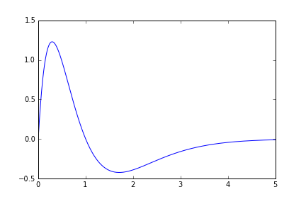
We use these functions and matplotlib to plot the original equation

from pylab import plot, show, legend
xx = linspace(0, 5, 50000)
plot(xx, fn_numpy(xx))

Performance

When we profile these functions we find that the Fortran solution runs a bit faster. This is because it is able to fuse all of the scalar operations into one loop while the numpy solution walks over memory several times, performing each operation individually. Jensen wrote a more thorough blogpost about this when he worked on code generation. He shows substantial performance increases as the complexity of the mathematical expression increases.

>>> timeit fn_numpy(xx)
1000 loops, best of 3: 1.4 ms per loop
>>> timeit fn_fortran(xx)
1000 loops, best of 3: 884 us per loop

This weekend I built up a translation from SymPy expressions to Theano computations. This builds off of old work done with Frederic Bastien at SciPy2012.

>>> from sympy.printing.theanocode import theano_function
>>> fn_theano  = theano_function([x], [expr], dims={x: 1}, dtypes={x: 'float64'})
>>> timeit fn_theano(xx)
1000 loops, best of 3: 1.04 ms per loop

Theano generates C code that performs the same loop fusion done in Fortran but it incurs a bit more startup time. It performs somewhere between the numpy and Fortran solutions.

However, the SymPy to Theano translation interface only takes up about a page of code while the lambdify and autowrap modules are substantially more complex. Additionally, Theano is actively developed and is sure to improve and track changes in hardware well into the future. lambdify and autowrap have been relatively untouched over the past year. For example Theano is able to seemlessly compile these computations to the GPU.

Leveraging Theano

In the above example we used Theano to copy the behavior of SymPy’s existing numpy and Fortran numeric solutions. Theano is capable of substantially more than this. To show a simple example we’ll compute both our original output and the derivative simultaneously.

outputs = expr, simplify(expr.diff(x))
print latex(outputs)

\[\begin{pmatrix}\frac{8}{3} x \left(- 4 x + 4\right) e^{- 2 x}, & \frac{32}{3} \left(2 x^{2} - 4 x + 1\right) e^{- 2 x}\end{pmatrix}\]

We redefine our functions to produce both outputs, instead of just expr alone

fn_numpy  = lambdify([x], outputs, 'numpy')
fn_theano = theano_function([x], outputs, dims={x: 1}, dtypes={x: 'float64'})

fns_fortran = [ufuncify([x], output) for output in outputs]
fn_fortran  = lambda xx: [fn_fortran(xx) for fn_fortran in fns_fortran]

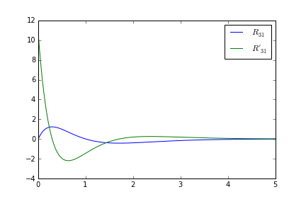
The expression and its derivative look like this:

for y in fn_theano(xx):
    plot(xx, y)
legend(['$R_{31}$', "$R'_{31}$"])

Because Theano handles common subexpressions well it is able to perform the extra computation with only a very slight increase in runtime, easily eclipsing either of the other two options.

>>> timeit fn_numpy(xx)
100 loops, best of 3: 2.85 ms per loop
>>> timeit fn_fortran(xx)
1000 loops, best of 3: 1.8 ms per loop
>>> timeit fn_theano(xx)
1000 loops, best of 3: 1.16 ms per loop

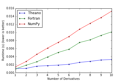
When we extend this experiment and vary the number of simultaneous derivatives we observe the following runtimes

In the case of highly structured computation Theano is able to scale very favorably.

Conclusion

The Theano project is devoted to code generation at a level that exceeds the devotion of SymPy to this same topic. This is natural and prevalent. When we combine the good parts of both projects we often achieve a better result than with an in-house solution

In-house solutions to foreign problems lack persistence. As programmers within an ecosystem we should make projects that do one thing well and provide clean interfaces and simple data structures to encourage inter-project communication.